Getting started
Introduction to Boolean Networks
Symbolic representation
Installing griffin
File interface
Using the API programmatically
References
Introduction to Boolean Networks
A Boolean Network \(BN\) is a formal model of a discrete dynamical system where a set of Boolean variables update their state according to a set of Boolean functions. That is \(BN = (V, F)\) where \(V = \{v_1, v_2, ..., v_N\}\) is the set of \(N\) propositional variables, \(v_i \in \mathbb{B}\), where \(\mathbb{B} = \{0,1\}\); and \(F = \{ f_1, f_2, ..., f_N\}\) the set of next-state functions, \(f_i:\mathbb{B}^N \to \mathbb{B}\). If \(b \in \mathbb{B}\), then \(b'\) is the complement of \(b\).
Assuming a fixed, increasing ordering of the propositional variables based on their subindex, a particular assignment of all variables is called a state and can be represented as a Boolean vector \(\bar{x} = (x_1, x_2, ..., x_N)\). Starting from a particular state \(\vec{x}^{(k)}\) at discrete time \(k\), the next state \(\vec{x}^{(k+1)}\) is given by \(\vec{x}^{(k+1)}= \vec{f}(\vec{x})=(f_1(\vec{x}^{(k)}), f_2(\vec{x}^{(k)}), ..., f_N(\vec{x}^{(k)}))\), where \(\vec{f}:\mathbb{B}^N \to \mathbb{B}^N\) is a Boolean vector function describing synchronous updating, i.e. all the variables update their value simultaneously.
For example, Given Boolean variables \(v_1\),\(v_2\) and \(v_3\) a synchronous Boolean function can be defined to describe the updating rule of each variable:
$$ \begin{align*} f_1(\vec{x}) &= x_1 \vee x_2\\ f_2(\vec{x}) &= \neg x_1\\ f_3(\vec{x}) &= x_1 \wedge \neg x_3 \end{align*} $$Starting from a particular state \(x\) at time 0, say \(\vec{x}^{(0)}=(0,1,1)\) the next state, or state at time 1, can be found by applying the updating rules
$$\vec{x}^{(1)}=F(0,1,1)=(0 \vee 1,\neg 0,0 \wedge \neg 1)=(1,1,0)$$ for time 2: $$\vec{x}^{(2)}=F(1,1,0)=(1 \vee 1,\neg 1,1 \wedge \neg 0)=(1,0,1)$$ and so on.Boolean Networks have been widely used to model Gene Regulatory Networks. Tipically, the propositional variables represent the activation state of a particular gene, product, or environmental signal (for the sake of brevity henceforward we will refer to the variables simply as "genes").
Gene Interaction Graph
Genes interact with each other according to the dynamics captured by \(\vec{f}\). Although, in principle each next-state function \(f_i\) can depend on all other genes of the network, it is often the case, that a particular gene depends only on a small subset of them, this subset is called its set of regulators. We can identify two types of regulators positive and negative.
Gene interactions are often represented by a Gene Interaction Graph \(G = (V, R^+,R^-)\) where \(V\) is the set of gene state variables, \(R^+ \subseteq V \times V\) is the set of positive regulations and \(R^- \subseteq V \times V\) the set of negative regulations. When depitcted, the network nodes (genes) are represented by circles, positive regulations are represented by lines with ordinary arrowheads \(\rightarrow\) showing the direction of the regulation (tip pointing towards the target gene) and negative interactions are represented by lines with flat arrowtips ( \(\dashv\) ) pointing towards the regulated gene. If \(x \in R^+ \cap R^-\), \(x\) is said to be an ambiguous regulation.

Steady States
Steady states are fixed points of the Boolean Network, that is \(\vec{x}^*\) is a steady state or fixed point if \(\vec{f}(\vec{x}^*) = \vec{x}^*\).
Fixed points are biologically relevant because they can represent particular cell types.
Cyclic Attractors
A state space trajectory of length \(L\) is a set of states \(\{\vec{x}_1,\vec{x}_2,...,\vec{x}_{L+1}\}\) satisfying \(\vec{x}_{i+1}= \vec{f}(\vec{x}_i)\).
Cyclic attractors are periodic state space trajectories. Formally: Given a state space trajectory \(\{\vec{x}_1,\vec{x}_2,...,\vec{x}_{T}\}\) where \(\vec{x}_i \neq \vec{x}_j\) for all \(i \neq j\) then if \(\vec{x}_i^{(k)} = \vec{x}_i^{(k+n T)}\) for \(i = 1,2,...,T\) and \(n = 1,2,3,...\), then all states in the trajectory form a cyclic attractor of length \(T\).
In the previous example the states \((1,0,0)\) and \((1,0,1)\) form a cyclic attractor of length 2. As can be seen from the network dynamics: $$F(1,0,0)=(1 \vee 0,\neg 1,1 \wedge \neg 0)=(1,0,1)$$ $$F(1,0,1)=(1 \vee 0,\neg 1,1 \wedge \neg 1)=(1,0,0)$$
Cyclic attractors can represent cell cycles or cyclic metabolic pathways.
Positional bindings and substitutions
Let \(\vec{x}=(x_1,x_2,\dots,x_N)\) be a Boolean vector. We write a positional binding as \(j/b\) with \(j \in \{1,2,\dots,N\}\) an index and \(b \in \mathbb{B}\) a Boolean value. A positional substitution is a set \(\sigma\) of positional bindings \(\sigma =\{j_1/b_1,j_2/b_2,\dots,j_K/b_K\}\) with \(K \in \{0,1,2,\dots,N\}\) and \(j_k \neq j_l\) for \(k \neq l\), if when applied to a Boolean vector \(\vec{x}\) denoted \(\vec{x}[\sigma]\), $$\vec{x}[\sigma] = (x_1',x_2',...,x_N') $$ where $$ x_i' = \begin{cases} x_i & i \notin Dom(\sigma)\\ b_k & \exists k. (i = j_k) \wedge (j_k/b_k \in \sigma) \end{cases} $$ and the domain \(Dom\) of the positional subsitution \(\sigma\), is defined as \(Dom(\sigma)=\{j_1,j_2,...,j_K\}\).
When writing \(\sigma\) explicitly as a set of bindings, the curly braces delimiting the set members are optional, for example we write \(\vec{x}[j_1/b_1,j_2/b_2]\) instead of \(\vec{x}[\{j_1/b_1,j_2/b_2\}]\). Also, we omit writing delimiters for singleton sets whenever doing this cannot lead to misinterpretation or ambiguity of sentences.
Mutant experiments
Mutation experiments alter the dynamics of the Boolean network by means of fixing the state of particular genes.
We represent a single mutation on the original \(BN = (V,F)\) as \(BN[{j/b}] = (V,F')\), where \(j/b\) is a positional binding and \(F' = \{f_1', f_2',...,f_N'\}\), \(j \in \{1,2,...,N\}\) and \(b \in \mathbb{B}\) where $$ f_i'(\vec{x}) = \begin{cases} b & i =j\\ f_i(\vec{x}) & otherwise \end{cases} $$
If \(b = 0\) the mutation is said to be a loss of function mutation, while if \(b = 1\) gain of function mutation.
Multiple mutations
Multiple mutations are simultaneous mutations, i.e. there are at least two genes for which either a gain of function or loss of function occurs.
In this case we represent a multiple mutation on the original \(BN = (V,F)\) as \(BN[\sigma] = (V,F')\), where \(\sigma\) is a positional substitution and \(F' = \{f_1', f_2',...,f_N'\}\), then for any state \(\vec{x}\) and \(\vec{f'}=(f_1', f_2',...,f_N')\) it will be true that $$ \vec{f'}(\vec{x}) = \vec{f}(\vec{x})[\sigma] $$ A single mutation is a particular case of the multiple mutation with \(\sigma\) the singleton set \(\{j/b\}\)
In our example performing a gain of function on \(v_1\) and a loss of function in \(v_3\) is expressed as $$ \vec{f'}(\vec{x}) = \vec{f}(\vec{x})[{1/1,3/0}] = (f_1',f_2,f_3') = (1,f_2(x),0) $$
Partial States
In a partial state there is at least one gene for which their Boolean value is unknown. In that sense, a partial state is a description of a set of states. To indicate that a given gene is unknown a wildcard symbol is used. For example the partial state \(\vec{x} = (1,*,*)\) describes the set of states \(\{(1,0,0),(1,0,1),(1,1,0),(1,1,1)\}\).
An alternative notation for the partial state is: $$ \langle \sigma,*\rangle = \{ \vec{x}[\sigma] \mid \vec{x} \in \mathbb{B}^N \} $$ for the previous example \((1,*,*) = \langle 1/1,*\rangle\)
Partial states define subspaces in the sense defined by Klarner and Siebert.
Symbolic representation
Griffin transforms the biological constraints in a propositional sentence. This section describes the way this sentence is built. This is not a comprehensive account of the formulas, nevertheless the list is representative. Griffin will do the automatic compilation of queries into large Boolean formulas. Readers not interested in the encoding can skip this section. Readers seeking a more detailed description of the methods are refered to the paper of Rosenblueth et al. (2014).
Propositional variables
It is important to note that Griffin does not perform operations in the domain of the gene state variables described in the previous sections. The variables to be assigned by the SAT engine are those that represent the update rules. A straightforward representation would be to use one variable per row in the truth table that describe the next state for each of the gene state variables. As it is assumed that the gene interaction graphs is known in advance, i.e. it is a biological constraint, then it can be shown that the minimum number of variables required to represent a Boolean function depends only on the effective regulators for each gene, the inclusion of other genes does not add any information.
Given the predecessor set (in-neighborhood) of a gene \(v_i\) in the interaction graph \(G=(V,R^+,R^-)\) as follows: $$ N_G^-(v_i) =\{v_j \mid (v_j,v_i) \in R^+ \cup R^-\} $$ and a total order of the gene state variables denoted as \(\leq_V\) then we define the set of function definition variables for the gene \(v_i\) as $$ U(v_i) = \{ v_{i,j} \mid j \in 0,1,...,2^{|N_G^-(v_i)|}-1\} $$ If we have a complete assignment \(\sigma_{U(v_i)}:U(v_i) \to \mathbb{B} \) for the function definition variables \(U(v_i)\) they will be related to the next-state function \(f_i\) of gene \(v_i\), as follows: $$ \sigma_{U(v_i)} \vDash f_i \leftrightarrow v_{i,j} \wedge (j = index(\sigma_{U(v_i)},\leq_V)) $$ here the function \(index:((2^V \to \mathbb{B}) \times 2^{V \times V}) \to \{0,\dots,2^{|N_G^-(v_i)|}-1\}\) relates an integer to the provided assignment \(\sigma_{U(v_i)}\)and ordering relation \(\leq_V\): $$ index(\sigma_{U(v_i)},\leq_V) = \sum_{v_j \in N_G^-(v_i)} 2^{|N_G^-(v_i)|-pos(v_j)}\sigma_{U(v_i)}(v_j) $$ where: $$ pos(v_i,\leq_V) = \begin{cases} 1 & \nexists u. u \in U(v_i) \wedge u \prec v_i \wedge u \neq v_i \\ n & \exists u. u \in U(v_i) \wedge u \prec v_i \wedge n = pos(u,\leq_V) + 1 \end{cases} $$ where \(a \prec b\) means \(a\) is the predecessor of \(b\) in the given ordering \(\leq_V\)
Consider for example the gene interaction graph of Fig. 1. If we were to find the update rule for the gene \(v_2\), then as there are only two regulators for this gene, \(v_1\) and \(v_3\) (\(v_2\) does not regulate itself), the corresponding truth table is given by:
| v1 | v3 | v2' |
| 0 | 0 | v2,0 |
| 0 | 1 | v2,1 |
| 1 | 0 | v2,2 |
| 1 | 1 | v2,3 |
The SAT engine will find a satisfying assignment for the function definition variables \(v_{2,0},v_{2,1},v_{2,2},v_{2,3}\), and by doing so, specifying the update function of gene \(v_2\). If now we consider the update rule for gene \(v_1\), we see that according to the interaction graph depitcted in Fig. 1, \(v_2\) is its only regulator, therefore the truth table can be expressed as follows:
| v2 | v1' |
| 0 | v1,0 |
| 1 | v1,1 |
A similar truth table can be defined for the update rule of gene \(v_3\) .
Regulation formula
We say that gene \(v_1\) regulates positively gene \(v_2\) if there exist at least one gene state configuration of all other regulators of \(v_2\), such that leaving them constant and changing the state of \(v_1\) from \(0\) to \(1\), changes the state of gene \(v_2\) from \(0\) to \(1\). Similarly, \(v_1\) regulates negatively gene \(v_2\) if there exist at least one gene state configuration of all other regulators of \(v_2\), such that leaving them constant and changing the state of \(v_1\) from \(0\) to \(1\), changes the state of gene \(v_2\) from \(1\) to \(0\).
Griffin includes explicit variables to represent gene regulations. We define the regulation variable \(R_{i,j}^+\) as representing that gene \(v_i\) positively regulates gene \(v_j\), and \(R_{i,j}^-\) representing gene \(v_i\) negatively regulates gene \(v_j\) as follows: $$ R_{i,j}^+ \leftrightarrow \bigvee_{k = 0}^{2^{|N_G^-(v_i)|}-1} \neg v_{i,r_{i,j,k}^0} \wedge v_{i,r_{i,j,k}^1} $$ $$ R_{i,j}^- \leftrightarrow \bigvee_{k = 0}^{2^{|N_G^-(v_i)|}-1} v_{i,r_{i,j,k}^0} \wedge \neg v_{i,r_{i,j,k}^1} $$ $$ r_{i,j,k}^0 = k \bmod 2^{|N_G^-(v_i)|-j} + \lfloor{k}/|N_G^-(v_i)|\rfloor 2^{|N_G^-(v_i)|-j+1} $$ $$ r_{i,j,k}^1 =r_{i,j,k}^0+ 2^{|N_G^-(v_i)|-j} $$
According to this interpretation, and using the propositional variables found in the previous section. The positive regulation of \(v_1\) in \(v_2\) ( \(R_{1,2}^+\) ) can be represented by the sentence:
Similarly the negative regulation of \(v_1\) in \(v_3\) ( \(R_{1,3}^-\) ) can be codified as:
The sentences corresponding to the remaining regulations are given by
Griffin encoding for the interaction graph in Fig. 1 is given by:
$$ \begin{aligned} \phi_{graph}(G) = ( R_{1,2}^+ &\leftrightarrow ( \neg v_{2,0} \wedge v_{2,2} ) \vee ( \neg v_{2,1} \wedge v_{2,3} ) ) \wedge \\ ( R_{3,2}^+ &\leftrightarrow ( \neg v_{2,0} \wedge v_{2,1} ) \vee ( \neg v_{2,2} \wedge v_{2,3} ) ) \wedge \\ ( R_{1,3}^- &\leftrightarrow v_{3,0} \wedge \neg v_{3,1} ) \wedge \\ ( R_{2,1}^+ &\leftrightarrow \neg v_{1,0} \wedge v_{1,1} ) \end{aligned} $$
The introduction of the regulation variables \(R_{i,j}^{+/-}\) will help to keep the encoding sentence small and define other biological constraints and hypotheses. In some cases a fully ambigous graph \(G_*=(V,R_*^+,R_*^-)\) is constructed where for every edge \((v_i,v_j) \in (R^+ \cup R^-)\) in \(G\), \((v_i,v_j) \in R_*^+\) and \((v_i,v_j) \in R_*^- \). The fully ambiguous graph will be useful to enforce certain constraints regarding ambiguous (double regulations, that is a positive and a negative regulation, from a source gene \(v_a\) to a target gene \(v_b\) ) and non ambiguous regulations.
Input-Output sentence
A pair of consecutive states \(\vec{x}^{(k)}\) and \(\vec{x}^{(k+1)}\) can be specified in Griffin as a biological constraint. Griffin encodes such constraint as follows:
Starting with the sentence \(\phi_{io} \leftarrow true\). For each gene \(v\): 1) lookup the corresponding next state variable \(v_{i,j}\) which is consistent with the provided state \(\vec{x}^{(k)}\). 2) If \(\vec{x}^{(k+1)}_{j} =1\) conjoin the literal \(v_{i,j}\) to \(\phi_{io}\), that is \(\phi_{io} \leftarrow \phi_{io} \wedge v_{i,j}\), 3) otherwise conjoin the literal \(\neg v_{i,j}\) to \(\phi_{io}\), that is \(\phi_{io} \leftarrow \phi_{io} \wedge \neg v_{i,j}\).
For example, if we want to encode the constraint given by \(\vec{x}^{(k)} = (0,1,0)\) and \(\vec{x}^{(k+1)} = (1,0,1) \) Starting with gene \(v_1\) we know its only regulator is \(v_2\), looking up at the truth table we find the only consistent row is that of \(v_{1,1}\) because it corresponds with \(\vec{x}^{(k)}_{2} = 1\). Also \(\vec{x}^{(k+1)}_{1} = 1\), therefore \(\phi_{io} \leftarrow true \wedge v_{1,1} \) For \(v_2\) we have two regulators \(v_1\) and \(v_3\), in this case the consistent variable is \(v_{2,0}\) because \(\vec{x}^{(k)}_{1} = 0\) and \(\vec{x}^{(k)}_{3} = 0\). In this case \(\vec{x}^{(k+1)}_{2} = 0\), thus \(\phi_{io} \leftarrow v_{1,1} \wedge \neg v_{2,0}\). Finally \(v_3\) only has \(v_1\) as regulator, the consistent variable is \(v_{3,0}\) because \(\vec{x}^{(k)}_{1} = 0\). Given that \(\vec{x}^{(k+1)}_{3} = 1\) we have \(\phi_{io} \leftarrow v_{1,1} \wedge \neg v_{2,0} \wedge v_{3,0}\) In this case the Input-Output sentence
To describe this formally we can give a name to each raw of the truth tables. For instance, in the truth table for \(v_2'\) we define the following:
$$\begin{aligned} \neg v_1 \wedge \neg v_3 &\leftrightarrow \hat{v}_{2,0} \\ \neg v_1 \wedge v_3 &\leftrightarrow \hat{v}_{2,1} \\ ...&\\ v_1 \wedge v_3 &\leftrightarrow \hat{v}_{2,3} \end{aligned}$$
Note that for a full assignment of the regulator variables of \(v_2\) there is exactly one variable \(\hat{v}_{2,i}\) which is true, all others will be false. In the case of a partial assignment of the regulator variables, a disjunction will be implied, for example if \(v_1 = 0\) then either \(\hat{v}_{2,0}\) or \(\hat{v}_{2,1}\) will be true.
A state \(\vec{x}\) relates to an assignment \(\sigma : V \to \mathbb{B}\) of the propositional variables as follows:
$$\sigma_{\vec{x}}(v_i) = x_i$$
It can be shown that exactly one \(\hat{v}_{i,j}\) variable is active at a given time for a given gene \(v_i\), that is:
therefore we define the variable selector function of a state \(\vec{x}\) and a gene \(v_i\) as the function \(\sigma_{\vec{x}}^{-1}(v_i): \mathbb{B}^N \times V \to U(v_i)\) as follows: $$\sigma_{\vec{x}}^{-1}(v_i) = v_{i,j} \leftrightarrow \hat{v}_{i,j}=true$$
If \(v\) is a propositional variable and \(b\in \mathbb{B}\), the literal of \((v,b)\) is defined as \(lit(v,b)=\neg v\) if \(b=0\) and \(lit(v,b)= v\) if \(b=1\).
The encoding of an Input-Output pair \((x,y)\) is then give by: $$\phi_{io}(x,y) = \bigwedge_{i} lit(\sigma_{\vec{x}}^{-1}(v_i),y_i)$$
Fixed point sentence
Adding constraints for known fixed points (steady states) in the dynamics of the Boolean network is simple $$\phi_{FP}(\vec{x}) \equiv \phi_{io}(\vec{x},\vec{x})$$
Mutantion formula
Encoding single mutations is computationally inexpensive. A sentence is added for each fixed point \(\vec{x}\) in the mutated Boolean network \(BN[j/b]\) that IS NOT a fixed point in the wild type network. Let \(A\) be the set of fixed points in the wild type network \(BN\), and \(B\) the set of fixed points in \(BN[j/b]\), then the encoding is given by the sentence: $$\phi_{mut}(A,B,j/b) \equiv \bigwedge_{\vec{x} \in (B-A)}\phi_{io}(\vec{x},\vec{x}[j/b'])$$
Multiple mutation formula
For the multiple mutation of the Boolean network given by \(BN[\sigma]\), \(A\) the set of fixed points of the wildtype network and \(B\) the set of fixed points of the mutated network, then encoding sentence is given by $$\phi_{mut}(A,B,\sigma) = \bigwedge_{\vec{x} \in (B-A)} {\left(\bigwedge_{i \notin Dom(\sigma)} lit(\sigma_{\vec{x}}^{-1}(v_i),x_i) \wedge \bigvee_{j/b \in \sigma} lit(\sigma_{\vec{x}}^{-1}(v_j),b')\right) } $$ Note that the multiple mutation sentence reduces to the single mutation when \(\sigma\) is a singleton set.
Partially defined Input-Output sentence
The encoding of a partially defined Input-Output pair \(( \langle \sigma_I,*\rangle, \langle \sigma_O,*\rangle)\) is given by: $$\phi_{io}( \langle \sigma_I,*\rangle, \langle \sigma_O,*\rangle) = \bigwedge_{\vec{x} \in \langle \sigma_I,*\rangle} \bigwedge_{i/b \in \sigma_O} lit(\sigma_{\vec{x}}^{-1}(v_i),b) $$
Multiple mutations with partially defined fixed points
As partially defined single mutations are a particular case of the multiple mutation sentence, only the latter will be given in this section. Also note that in the most general case the sets \(A\) and \(B\) of fixed points of the wildtype \(BN\) and the mutated \(BN[\sigma]\) networks will be a combination of completely defined and partial Boolean states. But because a fully specified state is a particular case of a partial state for which \(\left| \sigma\right| = N\), then without loss of generallity it will be considered than both \(A\) and \(B\) contain partial states as their members. In this case consider \(S = \{\langle \sigma_s,* \rangle \mid \forall_{a \in A}. {\langle \sigma_s,* \rangle \cap\ a = \varnothing \}} \) $$ \phi_{mut}(A,B,\sigma) = \bigwedge_{\langle \sigma_s,* \rangle \in S} \left[\bigvee_{\vec{x} \in \langle \sigma_s,* \rangle} {{\left(\bigwedge_{i \notin Dom(\sigma_s)} lit(\sigma_{\vec{x}}^{-1}(v_i),x_i) \wedge \bigvee_{j/b \in \sigma_s} lit(\sigma_{\vec{x}}^{-1}(v_j),b')\right) }}\right] $$
Hypotheses
Regarding the interaction graph, it may be the case that not all gene interactions are fully known in advance. Griffin allows for the incorporation of hypotheses, that is, it can add putative regulations to the encoding sentence. Since those constraints are optional, they can be called soft constraints, in the sense that Griffin won't necessarily enforce them, but they may become active if required.
The first thing to note about the description of our encoding method is that number and naming of function definition variables depend completely on the interaction graph, so that by construction it is impossible for Griffin to represent Boolean networks with additional regulations not present in the interaction graph, except perhaps for ambiguous ones. Therefore, in order to incorporate hypotheses, that is optional regulations, Griffin has to extend the set of regulators of a given gene with their putative (optional) regulators. Therefore the extended gene interaction graph is an interaction graph \( G'=(V,R^+,R^-)\) for wich positive hypothetical interactions \(H^+ \subseteq R^+\) and negative hypothetical interactions \(H^- \subseteq R^-\) are defined.
Queries
Queries can be stated using the presented encodings. Here we give some examples:
1. Find all networks that satisfy a given interaction graph \(G=(V,R^+,R^-)\), ignore hypothesis \(H^+\) and \(H^-\). $$ \phi_{query}(G) = \phi_{graph}(G) \wedge \left[ \bigwedge_{(i,j) \in (R^+ - H^+)} R^+_{i,j}\right] \wedge \left[ \bigwedge_{(i,j) \in (R^- - H^-)} R^-_{i,j} \right] $$ First thing to note here is that, strictly speaking, Griffin will not exclude networks with ambiguous regulations, even if they are not present in \(G\), unambiguous regulations must be explicitly prohibited.
2. Find all networks that satisfy a given interaction graph \(G=(V,R^+,R^-)\), ignore hypothesis \(H^+\) and \(H^-\) and exclude ambiguous regulations. $$ \phi_{query}(G) = \phi_{graph}(G_*) \wedge \left[ \bigwedge_{(i,j) \in (R^+ - H^+)} R^+_{i,j} \wedge \neg R^-_{i,j}\right] \wedge \left[ \bigwedge_{(i,j) \in (R^- - H^-)} R^-_{i,j} \wedge \neg R^+_{i,j} \right] $$ More complex queries can be constructed by conjoining the corresponding encodings for the required properties.
3. Find all networks \(BN\) that satisfy a given interaction graph \(G=(V,R^+,R^-)\), include all hypothesis \(H^+\) and \(H^-\), exclude ambiguous regulations. Include only those networks that have exactly the set of fixed points \(A\) in the wildtype state, but exclude those not consistent with the set of partial states \(B\) that are fixed points of the multiple mutation experiment in \(BN[\sigma]\) $$ \begin{align} \phi_{query}(G) =& \phi_{graph}(G_*) \wedge \left[ \bigwedge_{(i,j) \in R^+} R^+_{i,j} \wedge \neg R^-_{i,j}\right] \wedge \left[ \bigwedge_{(i,j) \in R^-} R^-_{i,j} \wedge \neg R^+_{i,j} \right] \wedge \\ &\left[ \bigwedge_{\vec{x} \in A} \phi_{FP}(\vec{x}) \wedge \bigwedge_{\vec{x} \in (\mathbb{B}^N-A)} \neg \phi_{FP}(\vec{x}) \right] \wedge \phi_{mut}(A,B,\sigma) \end{align} $$
Generalized interactions
The query examples given in the previous section, are based on the distinction of known and hypothetical regulations, and whether ambiguity is allowed or not in a global maner. A more refined approach to building queries would allow the researcher to ask for such properties in a gene to gene basis. Griffin allows the formulation of queries based on what is called generalized interactions. Given an ordered pair of genes \((v_i,v_j)\), a generalized interaction of \(v_i\) with \(v_j\) is defined as any Boolean function that can be defined for the combination of the regulation variables \(R_{i,j}^+\) y \(R_{i,j}^-\). As there are \(2^{2^n}\) possible functions, having \(n=2\) variables, we define \(16\) different gene interactions.
| \(R_{i,j}^+\) | \(R_{i,j}^-\) | \(\mathrm{I}_0\) | \(\mathrm{I}_1\) | \(\mathrm{I}_2\) | \(\mathrm{I}_3\) | \(\mathrm{I}_4\) | \(\mathrm{I}_5\) | \(\mathrm{I}_6\) | \(\mathrm{I}_7\) | \(\mathrm{I}_8\) | \(\mathrm{I}_9\) | \(\mathrm{I}_{A}\) | \(\mathrm{I}_{B}\) | \(\mathrm{I}_{C}\) | \(\mathrm{I}_{D}\) | \(\mathrm{I}_{E}\) | \(\mathrm{I}_{F}\) |
| 0 | 0 | 0 | 0 | 0 | 0 | 0 | 0 | 0 | 0 | 1 | 1 | 1 | 1 | 1 | 1 | 1 | 1 |
| 0 | 1 | 0 | 0 | 0 | 0 | 1 | 1 | 1 | 1 | 0 | 0 | 0 | 0 | 1 | 1 | 1 | 1 |
| 1 | 0 | 0 | 0 | 1 | 1 | 0 | 0 | 1 | 1 | 0 | 0 | 1 | 1 | 0 | 0 | 1 | 1 |
| 1 | 1 | 0 | 1 | 0 | 1 | 0 | 1 | 0 | 1 | 0 | 1 | 0 | 1 | 0 | 1 | 0 | 1 |
Where \(\mathrm{I_j}\) represent the type of the interaction. To facilitate the interpretation of such interactions, Griffin defines the following acronyms
| Interaction | Formula | Acronym | Meaning |
| \(\mathrm{I}_0\) | \(0\) | false | Contradiction |
| \(\mathrm{I}_1\) | \(R_{i,j}^+ \wedge R_{i,j}^-\) | MA | Mandatory, ambiguous |
| \(\mathrm{I}_2\) | \(R_{i,j}^+ \wedge \neg R_{i,j}^-\) | MPU | Mandatory, positive, unambiguous |
| \(\mathrm{I}_3\) | \(R_{i,j}^+\) | MPPA | Mandatory, positive, possibly ambiguous |
| \(\mathrm{I}_4\) | \(\neg R_{i,j}^+ \wedge R_{i,j}^-\) | MNU | Mandatory, negative, unambiguous |
| \(\mathrm{I}_5\) | \(R_{i,j}^-\) | MNPA | Mandatory, negative, possibly ambiguous |
| \(\mathrm{I}_6\) | \(\neg(R_{i,j}^+ \leftrightarrow R_{i,j}^-)\) | MUSU | Mandatory, unknown sign, unambiguous |
| \(\mathrm{I}_7\) | \(R_{i,j}^+ \vee R_{i,j}^-\) | MUSPA | Mandatory, unknown sign, possibly ambiguous |
| \(\mathrm{I}_8\) | \(\neg (R_{i,j}^+ \vee R_{i,j}^-)\) | NR | No regulation |
| \(\mathrm{I}_9\) | \((R_{i,j}^+ \leftrightarrow R_{i,j}^-)\) | OA | Optional, ambiguous |
| \(\mathrm{I}_{A}\) | \(\neg R_{i,j}^-\) | OPU | Optional, positive, unambiguous |
| \(\mathrm{I}_{B}\) | \(R_{i,j}^+ \vee \neg R_{i,j}^-\) | OPPA | Optional, positive, possibly ambiguous |
| \(\mathrm{I}_{C}\) | \(\neg R_{i,j}^+\) | ONU | Optional, negative, unambiguous |
| \(\mathrm{I}_{D}\) | \(\neg R_{i,j}^+ \vee R_{i,j}^-\) | ONPA | Optional, negative, possibly ambiguous |
| \(\mathrm{I}_{E}\) | \(\neg(R_{i,j}^+ \wedge R_{i,j}^-)\) | OUSU | Optional, unknown sign, unambiguous |
| \(\mathrm{I}_{F}\) | \(1\) | true | Tautology |
The generalized interaction space can be visualized in the following depiction

Installing griffin
Griffin can be used as a command line tool or as an application programming interface (java API).
To start using Griffin it is required to have java Runtime Environment installed. We recommend you to use Oracle's Standard Edition JDK 1.8.x if you wish to use Griffin programmatically.
To test you have correctly installed java, try running the following command from a terminal
java -version
You should be seeing something like the following:

Once you have installed java Runtime Environment, download Griffin project file from here. Unpack the contents of the archive by running
tar -xzvf griffin-0.1.5.tar.gz

Your installation include 12 directories, as you can see in the following screenshot

Make sure Griffin scripts have execution privileges by running
chmod +x *griffin*

export GRIFFIN_HOME=/home/stan/griffin-0.1.5
export PATH=$PATH:$GRIFFIN_HOME
export GRIFFIN_JVM_OPTIONS="-XX:-UseGCOverheadLimit \
                            -Xmx15000m -XX:-UseConcMarkSweepGC"
The variable GRIFFIN_JVM_OPTIONS are parameters for the java virtual machine.
In my case the parameter -Xmx15000m sets the maximum heap size to 15GB of RAM.
Change this option to appropriate values according to your computer resources and needs.
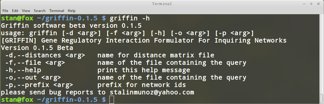
Finally, test your installation by typing
griffin -h
You should be seeing the following output on the screen
System requirements
| Feature | Requirement |
| Operative System | Currently Griffin has only been tested on Linux 64 bit distributions. But as it was developed using java, it is expected to run on several platforms. |
| Java | Compatible with Java 1.8. Griffin has been only tested with Oracles's Java (TM) SE Runtime Environment 1.8.x |
| Hard Drive | No minimal hard drive requirement. |
| RAM Memory | 2GB. Depending on the query, finding all satisfying models may consume a considerable amount of RAM, we recomend 16GB or more for complex queries. |
External dependencies
| Library | Version |
| Java BeeDeeDee Library | 1.0.7 |
| Commons BeanUtils | 1.8.x |
| Commons BeanUtils Bean Collection | 1.8.x |
| Commons BeanUtils Core | 1.8.x |
| Commons CLI | 1.2.x |
| Commons Lang | 3.3.x |
| Log4j | 1.2.x |
| SAT4j Core | 2.3.4 |
| Efficient Java Matrix Library | 0.2.9 |
File interface
Griffin provides with a basic query file interface. To generate a query using this interface, there is no need to compile or do any programming. The syntax of the query will be illustrated using examples.
Examples
Akutsu, Miyano y Kuhara 3 genes example
Consider the interaction graph of Fig. 1. A very simple query would be to enumerate all networks satisfying the provided gene regulations. We will allow cyclic, as well as fixed points attractors to occur. Nevertheless, we will not constraint them to especific values. Also we ask Griffin to exclude ambiguous regulations. In this query there are no hypothesis to test. The input file describing this query is:
#Akutsu, T., Miyano, S., & Kuhara, S. (1999, January).
#Identification of genetic networks from a small number of gene expression patterns under the Boolean network model.
#In Pacific symposium on biocomputing (Vol. 4, pp. 17-28).
#Name and order of nodes
genes={v1,v2,v3}
#Regulations
known = {v1->v2,v1-|v3,v2->v1,v3->v2}
#options
allow.ambiguity = false
allow.additional.states = true
allow.additional.cycles = true
allow.hypotheses = true
block.steady.a.posteriori = false
divide.query.by.topology = false
As can be seen, the input file can include comments. Comments are any line starting with the number sign #. To specify the names of the genes this is done using the keyword genes then the symbol equals followed by a list of gene names. Gene names should start with a letter cannot include spaces or blank characters, can include numbers and single underscores. Double underscores are reserved and should not be used. Forward slash is allowed too. No other characters can be used as gene names. Examples of valid identifiers are A1,IAA, CDK_2/CYE_1. Examples of invalid identifiers are 1A, A__3, B-2, CDK+. Griffin experimental file parser, is not strict, and will ignore invalid characters. Care must be taken to avoid input errors by the user.
Known regulations are specified using the keyword known followed by equals
sign and a list of regulations. Positive
regulations are specified using the operator \(->\) (hyphen followed by bigger than symbol),
while negative regulations
are writen as \(-|\) (hyphen followd by pipe symbol).
In the example \(v1 -> v2\) means \(v_1\) positively regulates \(v_2\),
and \(v1 -| v3\) than \(v_1\) negatively regulates \(v_3\).
The Boolean flags under the comment options specify that ambiguous regulations are allowed.
Additional steady states to those specified (in this case none),
and cyclic attractors are okay.
To run the query we will create a new text file with the code provided and give it
the name akutsu.grf.
Assuming we have included the script in our path we can simply run the command:
griffin -f akutsu.grf -o akutsu.out
As can be seen in figure 8, Griffin finds two satisfying Boolean networks to the query. The anser to the query is in file "akutsu.out". It contains two lines. One for each answer. Each line contains several fields, each separated by a comma. The first field is an id, in this case 0000000000 and 0000000001 for the first and second network, respectively. The second field is the number of genes, in this case 3. The third field is the list of gene names, semicolon is used as separators within fields. The fourth field are the Boolean functions found by Griffin. In this case this field looks like this:
v2;(((~v1&v3)|(v1&~v3))|(v1&v3));~v1It means that the update rules for the genes are given by: $$ F=(v_2,(((\neg v_1 \wedge v_3)\vee(v_1\wedge \neg v_3))\vee(v_1 \wedge v_3)),\neg v_1) $$ The fifth field are the right hand side of the truth tables for the problem
01;0111;10| v2 | v1' |
| 0 | \(v_{1,0}=0\) |
| 1 | \(v_{1,1}=0\) |
| v1 | v3 | v2' |
| 0 | 0 | \(v_{2,0}=0\) |
| 0 | 1 | \(v_{2,1}=1\) |
| 1 | 0 | \(v_{2,2}=1\) |
| 1 | 1 | \(v_{2,3}=1\) |
| v1 | v3' |
| 0 | \(v_{3,0}=1\) |
| 1 | \(v_{3,1}=0\) |
v1+v2;v1-v3;v2+v1;v3+v2Now we will change the query slightly asking for those networks that don't have cyclic attractors. Again the file akutsu.grf should look like
#Akutsu, T., Miyano, S., & Kuhara, S. (1999, January).
#Identification of genetic networks from a small number of gene expression patterns under the Boolean network model.
#In Pacific symposium on biocomputing (Vol. 4, pp. 17-28).
#Name and order of nodes
genes={v1,v2,v3}
#Regulations
known = {v1->v2,v1-|v3,v2->v1,v3->v2}
#options
allow.ambiguity = false
allow.additional.states = true
allow.additional.cycles = false
allow.hypotheses = true
block.steady.a.posteriori = false
divide.query.by.topology = false
Note that the only property that has change is that of allow.additional.cycles which has been set to false.

Griffin has found zero satisfying models (the output file is empty). If we would like Griffin to give us more information about the conclusion, we can inspect the log file grn.log which is available in the directory log. Additionally we can choose to send the log information to the console this is achieved by modifying the file log4j.properties found in the GRIFFIN_HOME/conf directory.
# RAIZ
#log4j.rootLogger=DEBUG, file
log4j.rootLogger=INFO, file, stdout
Now when running the query we have more information about the resolving process

The level of detail can be changed by modifying the logging level INFO. For more information see Log4j documentation
Azpeitia et al. Arabidopsis thaliana root stem cell niche
A. thaliana root stem cell niche model of Azpeitia et al. (2010) is used to illustrate a more interesting query provided to Griffin. Figure 10 shows the interaction graph for this model. We can see some dashed edges that represent hypothetical regulations.

The model has the following gene variables: $$ \begin{equation*} V=\{SHR, SCR, JKD, MGP, PLT, IAA, AUX, ARF, WOX, CLE\} \end{equation*} $$
It is desired that the model recovers 5 known wild-type fixed-point attractors. Considering the previous ordering of the variables, the set of known attractors are: $$ \begin{equation*} \begin{split} A =& \{\{0000101100\}, \{1000101100\}, \{1000101101\},\\ &\{1110101110\}, \{1111101101\}\} \end{split} \end{equation*} $$
The query file is as follows:
# Model:
# Azpeitia, E, Benítez, M, Vega, I, Villarreal, C, Alvarez-Buylla, E R (2010).
# Single-cell and coupled GRN models of cell patterning in the Arabidopsis
# thaliana root stem cell niche. BMC systems biology, 4(1), 134.
#
# Query as formulated in, with no mutations:
# Rosenblueth, D. A., Muñoz, S., Carrillo, M., & Azpeitia, E. (2014, July).
# Inference of Boolean networks from gene interaction graphs using a SAT solver.
# In International Conference on Algorithms for Computational Biology
# (pp. 235-246). Springer International Publishing.
#
# Name and order of nodes
#
genes={SHR, SCR, JKD, MGP, PLT, IAA, AUX, ARF, WOX, CLE}

#
#Known regulations
#
known = {SHR->JKD,SHR->SCR,SHR->MGP,SHR->WOX,SCR->SCR,SCR->JKD,SCR->WOX,SCR->MGP,IAA-|ARF,AUX-|IAA,ARF->PLT,ARF->WOX,WOX-|MGP,CLE-|WOX}

#
#Hypothetical regulations
#
hypothetical = {SHR->SHR,SHR->CLE,CLE->CLE,MGP-|SCR,JKD->SCR}

#
# Fixed points, wild type
#
fixed-points()={1111101101,1000101101,1110101110,1000101100,0000101100}

# Options
allow.ambiguity = false
allow.additional.states = false
allow.additional.cycles = false
allow.hypotheses = true
block.steady.a.posteriori = false
divide.query.by.topology = false
As can be seen in the query, the hypothetical interactions are defined using the reserved word hypothetical. To activate hypotheses is required to set the option allow.hypotheses to true. The set of wild type steady states are defined usign the reserved word fixed-points. Here round brackets ( ) are important. The options of the query ask for non ambiguous regulations. Additional steady states are prohibited by setting allow.additional.states to false. Also we are prohibiting cyclic attractors by setting allow.additional.cycles to false.
To run the query we set first disable console logging by modifying the logging options in log4j.properties file:
# RAIZ
#log4j.rootLogger=DEBUG, file
log4j.rootLogger=INFO, file
Save the query in a file named azpeitia-2010-no-mutations.grf. To run the query type:
griffin -f azpeitia-2010-no-mutations.grf -o azpeitia-2010-no-mutations.out
We can use the command line wc in linux to obtain the number of lines in the output file, that is the number of satisfying Boolean networks.
In this case Griffin found 68. Figure 11 shows the result of these steps.

As seen in the previous section, the number of attractors is specified in the sixth field. In linux we can use the cut command to extract the attractors information from the output file, then passing the output to the command uniq that will delete repeated rows. As we expect 5 attractors we extract columns 6 to 16, Figure 12 shows this.
cut -d "," -f6-16 azpeitia-2010-no-mutations.out | uniq

In the previous example we can relax the constraint of prohibiting cyclic attractors by editing the query and setting allow.additional.cycles to true. In this case the number of satisfying networks is 74. That means that Griffin finds 4 Boolean networks that have cyclic attractors. We can use linux commands cut, sort and uniq to obtain a list of the number of attractors in the satisfying Boolean networks. Combinaning cat,grep,cut,sort and uniq we can list such attractors. The following commands do this:
#after allowing additional cycles the number of Boolean networks is 74
wc -l azpeitia-2010-no-mutations.out
# cut extracts the number of attractors, then the different numbers are found
cut -d "," -f6 azpeitia-2010-no-mutations.out | sort | uniq
# extracting attractors for Boolean networks with 7 attractors
cat azpeitia-2010-no-mutations.out | \
grep "[^,]*,[^,]*,[^,]*,[^,]*,[^,]*,7," | cut -d "," -f6-20 | sort | uniq
Figure 13 shows the previous command outputs. It can be seen that the 4 additional Boolean networks found by Griffin all have the same cyclic and fixed-point attractors. The cyclic attractors are: {1011101101,1100101101} and {1011101110,1100101100}.

We know proceed to prohibit cyclic attractors and will add constraints on the mutants. Griffin allows to specify the expected fixed point attractors after mutation. For example if we know that the fixed points after loss of function of gene SHR are reduced to the state {0000101100} then the syntax to specify this is as follows:
# the symbol ~ is used to define loss of function of a gene
fixed-points(~SHR) = {0000101100}
Gain of function for gene SCR will result in three steady states {0100101100,1110101110,1111101101}. The syntax to add the constraint is:
# For gain of function we simply mention the gene to mutate between the round brackets
fixed-points(SCR)={0100101100,1110101110,1111101101}
Here is the query that include all 20 mutations used in Rosenblueth et al. (2014):
# Model:
# Azpeitia, E, Benítez, M, Vega, I, Villarreal, C, Alvarez-Buylla, E R (2010).
# Single-cell and coupled GRN models of cell patterning in the Arabidopsis
# thaliana root stem cell niche. BMC systems biology, 4(1), 134.
#
# Query as formulated in:
# Rosenblueth, D. A., Muñoz, S., Carrillo, M., & Azpeitia, E. (2014, July).
# Inference of Boolean networks from gene interaction graphs using a SAT solver.
# In International Conference on Algorithms for Computational Biology
# (pp. 235-246). Springer International Publishing.
#
# Name and order of nodes
#
genes={SHR, SCR, JKD, MGP, PLT, IAA, AUX, ARF, WOX, CLE}

#
#Known regulations
#
known = {SHR->JKD,SHR->SCR,SHR->MGP,SHR->WOX,SCR->SCR,SCR->JKD,SCR->WOX,SCR->MGP,IAA-|ARF,AUX-|IAA,ARF->PLT,ARF->WOX,WOX-|MGP,CLE-|WOX}

#
#Hypothetical regulations
#
hypothetical = {SHR->SHR,SHR->CLE,CLE->CLE,MGP-|SCR,JKD->SCR}

#
# Fixed points, wild type
#
fixed-points()={1111101101,1000101101,1110101110,1000101100,0000101100}

#
# Mutant experiments loss-of-function mutations, single genes
#
#MGP loss-of-function experiment
fixed-points(~SHR)={0000101100}
#SCR loss-of-function experiment
fixed-points(~SCR)={0000101100,1000101100,1000101101}
#JKD loss-of-function experiment
fixed-points(~JKD)={0000101100,1000101100,1100101110,1000101101,1101101101}
#MGP loss-of-function experiment
fixed-points(~MGP)={0000101100,1000101100,1110101110,1000101101,1110101101}
#PLT loss-of-function experiment
fixed-points(~PLT)={0000001100,1000001100,1110001110,1000001101,1111001101}
#IAA loss-of-function experiment
fixed-points(~IAA)={0000101100,1000101100,1110101110,1000101101,1111101101}
#AUX loss-of-function experiment
fixed-points(~AUX)={0000010000,1000010000,1111010000,1000010001,1111010001}
#ARF loss-of-function experiment
fixed-points(~ARF)={0000001000,1000001000,1111001000,1000001001,1111001001}
#WOX loss-of-function experiment
fixed-points(~WOX)={0000101100,1000101100,1111101100,1000101101,1111101101}
#CLE loss-of-function experiment
fixed-points(~CLE)={0000101100,1000101100,1110101110}

#
# Mutant experiments gain-of-function mutations, single genes
#
#MGP gain-of-function experiment
fixed-points(SHR)={1000101100,1110101110,1000101101,1111101101}
#SCR gain-of-function experiment
fixed-points(SCR)={0100101100,1110101110,1111101101}
#JKD gain-of-function experiment
fixed-points(JKD)={0010101100,1010101100,1110101110,1010101101,1111101101}
#MGP gain-of-function experiment
fixed-points(MGP)={0001101100,1001101100,1111101110,1001101101,1111101101}
#PLT gain-of-function experiment
fixed-points(PLT)={0000101100,1000101100,1110101110,1000101101,1111101101}
#IAA gain-of-function experiment
fixed-points(IAA)={0000011000,1000011000,1111011000,1000011001,1111011001}
#AUX gain-of-function experiment
fixed-points(AUX)={0000101100,1000101100,1110101110,1000101101,1111101101}
#ARF gain-of-function experiment
fixed-points(ARF)={0000101100,1000101100,1110101110,1000101101,1111101101}
#WOX gain-of-function experiment
fixed-points(WOX)={0000101110,1000101110,1110101110,1000101111,1110101111}
#CLE gain-of-function experiment
fixed-points(CLE)={0000101101,1000101101,1111101101}

# Options
allow.ambiguity = false
allow.additional.states = false
allow.additional.cycles = false
allow.hypotheses = true
block.steady.a.posteriori = false
divide.query.by.topology = false
As can be seen in Figure 13, there are only 3 satisfying Boolean networks for the query.

The 3 Boolean networks found have the following update functions:
$$ \begin{equation*} \begin{split} F_1 =& (\\ &\text{SHR},\\ &\text{SCR}\wedge\text{SHR},\\ &\text{SCR}\wedge\text{SHR},\\ &\text{SCR}\wedge\text{SHR}\wedge \neg \text{WOX},\\ &\text{ARF}, \\ &\neg{AUX},\\ &1, \\ &\neg{IAA},\\ &\text{SCR}\wedge \text{ARF}\wedge \neg\text{CLE}\wedge\text{SHR},\\ &\text{CLE} \wedge \text{SHR}) \\ F_2 =& (\\ &\text{SHR},\\ &(\text{SCR}\wedge\neg\text{JKD} \wedge\neg\text{MGP}\wedge{SHR}) \vee(\text{SCR}\wedge\neg\text{JKD} \wedge\text{MGP}\wedge\text{SHR}) \\ &\vee(\text{SCR}\wedge\text{JKD}\wedge\neg\text{MGP} \wedge\neg\text{SHR}) \vee(\text{SCR}\wedge\text{JKD}\wedge\neg\text{MGP} \wedge\text{SHR}),\\ &\text{SCR}\wedge\text{SHR},\\ &\text{SCR}\wedge\text{SHR}\wedge \neg \text{WOX},\\ &\text{ARF}, \\ &\neg{AUX},\\ &1, \\ &\neg{IAA},\\ &\text{SCR}\wedge \text{ARF}\wedge \neg\text{CLE}\wedge\text{SHR},\\ &\text{CLE} \wedge \text{SHR}) \\ F_3 =& (\\ &\text{SHR},\\ &(\text{SCR}\wedge\neg\text{JKD}\wedge\text{SHR}) \vee (\text{SCR}\wedge \text{JKD}\wedge\neg\text{SHR}) \vee (\text{SCR}\wedge\text{JKD}\wedge\text{SHR}),\\ &\text{SCR}\wedge\text{SHR},\\ &\text{SCR}\wedge\text{SHR}\wedge \neg \text{WOX},\\ &\text{ARF}, \\ &\neg{AUX},\\ &1, \\ &\neg{IAA},\\ &\text{SCR}\wedge \text{ARF}\wedge \neg\text{CLE}\wedge\text{SHR},\\ &\text{CLE} \wedge \text{SHR}) \\ \end{split} \end{equation*} $$Using the API programmatically
Under construction
References
- Akutsu, T., Miyano, S., & Kuhara, S. (1999, January). Identification of genetic networks from a small number of gene expression patterns under the Boolean network model. In Pacific symposium on biocomputing (Vol. 4, pp. 17-28).
- Klarner, H., & Siebert, H. (2015). Approximating Attractors of Boolean Networks by Iterative CTL Model Checking. Frontiers in Bioengineering and Biotechnology, 3, 130. http://doi.org/10.3389/fbioe.2015.00130
- Rosenblueth, D. A., Muñoz, S., Carrillo, M., & Azpeitia, E. (2014, July). Inference of Boolean networks from gene interaction graphs using a SAT solver. In International Conference on Algorithms for Computational Biology (pp. 235-246). Springer International Publishing. https://link.springer.com/chapter/10.1007/978-3-319-07953-0_19#page-1
- Azpeitia, E., Benítez, M., Vega, I., Villarreal, C., & Alvarez-Buylla, E. R. (2010). Single-cell and coupled GRN models of cell patterning in the Arabidopsis thaliana root stem cell niche. BMC systems biology, 4(1), 134. https://bmcsystbiol.biomedcentral.com/articles/10.1186/1752-0509-4-134