Region growing

The region growing algorithm we use is based on an iterative relaxation technique. The classification of pixels as vessel or background is based primarily upon the maximum principal curvature $\kappa$, from which the criteria for determining seeds are defined. Using spatial information from the classification of the 8-neighbouring pixels, classes grow initially in regions with low gradient magnitude, $\gamma$, allowing a relatively broad and fast classification while suppressing classification in the edge regions where the gradients are large. In a second stage the classification constraint is relaxed and classes grow based solely upon $\kappa$ to allow the definition of borders between regions.

Figure 8: Parameters used in the region growing algorithm. (a) Histogram of the local maxima of the gradient magnitude strength, $\gamma$. One class: low gradient, $\gamma < \mu _{g} + \sigma _{g}$. (b) Histogram of the local maxima of the maximum principal curvature strength, $\kappa$, where $t$ is the threshold. Two classes: background, $\kappa /\kappa _{max} \in [0,t]$ and vessel, $\kappa /\kappa _{max} \in (t,1]$.

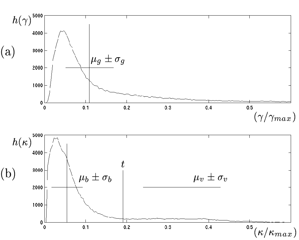
The histograms of both features $h(\gamma)$ and $h(\kappa)$ are calculated and for $h(\gamma)$ only one class is used: low gradient, which is defined as $\gamma < \mu _{g} + \sigma _{g}$ for the complete histogram (Figure 8(a)), where $\mu_{g}$ is the mean and $\sigma_{g}$ is the standard deviation. $h(\kappa)$ is automatically divided into two classes using the Otsu threshold algorithm [22], and their means and standard deviations are calculated: background, for $\kappa /\kappa _{max} \in [0,t]$ with mean $\mu_{b}$ and standard deviation $\sigma_{b}$ ; and vessel, for $\kappa /\kappa _{max} \in (t,1]$ with mean $\mu_{v}$ and standard deviation $\sigma_{v}$, where $t$ is the threshold (Figure 8(b)). The size of the interval for each class varies depending on the value of a parameter $a$, which changes during the iteration process. Intervals for each class are defined as: $\mu \pm a \sigma$.

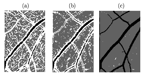
The algorithm begins by planting seeds for each region: background seeds are pixels for which $\kappa \le \mu_{b}$, whereas vessel seeds are defined as $\kappa \ge \mu_{v}$. Figure 9(a) shows an example of the planting stage where vessel seeds are shown in black, background seeds in gray and unknown pixels in white.

Figure 9: Region growing algorithm. (a) Planting seeds: black vessel seeds; gray, background seeds and white, unknown pixels. Two stages of region growing where information of the 8-neighbouring pixels is used. (b) Stage one: growth is restricted to regions with low gradients, allowing vessels to grow where the values of $\kappa$ lie within a wide interval and (c) stage two: classes grow without the gradient restriction to define borders between classes.

Region growing is an iterative process: An unlabelled pixel is classified as belonging to class $i$ if it has at least one neighbour of class $i$ already classified and if it fulfils a specific condition with initial parameters $a_{i}$=1. $a_i$ will specify the size of the class interval for the iteration $i$. Growing is repeated from left to right and top to bottom until no more pixels are classified. The constraints are relaxed by incrementing the parameters $a_{i}$ in steps of 0.5 and the growing is repeated.

In the first stage, the growing for both classes is restricted to regions with low gradients allowing rapid growth of regions outside of the boundaries, and allowing vessels to grow where the values of $\kappa$ lie within a wide interval. The condition for class vessel is:

$$(\mu_{v} - a_{v} \sigma_{v}) \leq \kappa \;\; \mbox{AND} \;... ...(\mu_{g} + a_{g} \sigma_{g}) \;\; \mbox{AND} \;\; N_{v} \geq 1$$ (6)

and for class background:

$$\kappa \leq (\mu_{b} + a_{b} \sigma_{b}) \;\; \mbox{AND} \;\; \gamma \leq \mu_{g} \;\; \mbox{AND} \;\; N_{b} \geq 1$$ (7)

where $N_{i}$ is the number of neighbours already labelled as class $i$. Figure 9(b) shows the result of the first stage after the restricted growing.

After alternating these two steps until no further classifications are found, the final stage of the algorithm grows vessel and background classes simultaneously without the gradient restriction. Now the condition for class $i$ is:

$$(\mu_{i} - a \sigma_{i}) \leq \kappa \leq (\mu_{i} + a \sigma_{i})\;\; AND\;\; N_{i} \geq 1$$ (8)

and again the condition is relaxed by increasing the value of $a=1$ by steps of 0.5 until all pixels are classified. With this final stage, borders between classes are defined. Figure 9(c) shows the result of the growing after this second stage.